R for Perl Hackers
Ladies and gentlemen, welcome to the
DISCLAIMER
R?
R is a programming language and software environment for statistical computing and graphics. The R language is widely used among statisticians and data miners for developing statistical software and data analysis. Polls, surveys of data miners, and studies of scholarly literature databases show that R's popularity has increased substantially in recent years.
R is an implementation of the S programming language combined with lexical scoping semantics inspired by Scheme. S was created by John Chambers while at Bell Labs. There are some important differences, but much of the code written for S runs unaltered.
R was created by Ross Ihaka and Robert Gentleman at the University of Auckland, New Zealand, and is currently developed by the R Development Core Team, of which Chambers is a member. R is named partly after the first names of the first two R authors and partly as a play on the name of S.
R is a GNU project. The source code for the R software environment is written primarily in C, Fortran, and R. R is freely available under the GNU General Public License, and pre-compiled binary versions are provided for various operating systems. R uses a command line interface; there are also several graphical front-ends for it.
Environment
sudo apt-get install r-base; R- Optional IDE (RStudio)
- Help: "
help(something)" or "?something" - Example data:
data() - Plotting included
R Language
- Impure functional
- Interpreted
- Weakly typed
- Lexically scoped
- Everything is an object
x <- 'lerele''larala' -> y
Data Types
- Atomic classes: numeric, logical, character, integer, complex
- Missing values
- Vectors and Matrices
- Factors
- Data frames
Data Types: Missing Values
- NA
- Nan (0/0)
Data Types: Vectors
Vectors contain elements of the same type
> x <- c(1,2,3,4)
> x
[1] 1 2 3 4

> y <- 1:32
> y
 [1]  1  2  3  4  5  6  7  8  9 10 11 12 13 14 15 16 17 18 19 20 21 22 23 24 25
[26] 26 27 28 29 30 31 32
Data Types: Vectors
Vector arithmetics
> x <- 1:10 > x * 2[1] 2 4 6 8 10 12 14 16 18 20
Data Types: Vectors
Vector arithmetics
> 10:1 + 1:10[1] 11 11 11 11 11 11 11 11 11 11
Data Types: Vectors
Vector arithmetics
> c(1,2,3,4) + c(0,10)[1] 1 12 3 14
Data Types: Vectors
Vector slicing
> x <- 1:10
> x > 3
 [1] FALSE FALSE FALSE  TRUE  TRUE  TRUE  TRUE  TRUE  TRUE  TRUE
> x[x > 3]
[1]  4  5  6  7  8  9 10
Data Types: Vectors
Vector access
> x <- (1:10)

> x[3]
[1] 3

> x[83]
[1] NA

> x[4] <- 3
> x
 [1]  1  2  3  3  5  6  7  8  9 10
Data Types: Matrices
Multi-dimension vectors
> m <- 1:10

> m
[1] 1 2 3 4 5 6 7 8 9 10

> dim(m) <- c(2, 5)

> m
     [,1] [,2] [,3] [,4] [,5]
[1,]    1    3    5    7    9
[2,]    2    4    6    8   10
Data Types: Factors
Represent categories ("labeled lists")
> x <- factor(c("yes", "yes", "no", "yes", "no"))

> x
[1] yes yes no yes no
Levels: no yes

> table(x)
x
no yes
 2   3

> unclass(x)
[1] 2 2 1 2 1
attr(,"levels")
[1] "no"  "yes"
Data Types: Data frames
List where every element of the list have a name and the same length
> x <- data.frame(foo = 1:4, bar = c(T, T, F, F))
> x
  foo   bar
1   1  TRUE
2   2  TRUE
3   3 FALSE
4   4 FALSE

> nrow(x)
[1] 4

> ncol(x)
[1] 2
Data Types: Data frames
> x <- data.frame(foo = 1:4, bar = c(T, T, F, F))

> x$foo
[1] 1 2 3 4

> x[,'foo']
[1] 1 2 3 4

> x[1,'foo']
[1] 1

> x[1,]
  foo  bar
1   1 TRUE
Data Types: Data frames
> x <- data.frame(foo = 1:10, bar = 100:109)

> x[5:6,]
  foo bar
5   5 104
6   6 105

> x[5:6,'bar']
[1] 104 105
Objects
attributes()
- names, dimnames
- dimensions (e.g. matrices, arrays)
- class
- length
- Attributes
> Marc$promise('MoreOnObjects')
Flow Control
if-else> w <- 3
> if (w < 5) {
d <- 2
} else if (w < 10) {
d <- 10
} else {
d <- 50
}
> d
2Flow Control
forx <- c("a", "b", "c", "d")
for(i in 1:4) {
print(x[i])
}
for(i in seq_along(x)) {
print(x[i])
}
for(letter in x) {
print(letter)
}
for(i in 1:4) print(x[i])Flow Control
whilez <- 5
while(z >= 3 && z <= 10) {
print(z)
coin <- rbinom(1, 1, 0.5)
if(coin == 1) { ## random walk
z <- z + 1
} else {
z <- z - 1
}
}Flow Control
repeat, next, returnFunctions
> x = function() { print('hi') }

> x
function() { print('hi') }

> x()
[1] "hi"
Functions
Signatures!!!
> args(lm)
function (formula, data, subset, weights, na.action, method = "qr",
    model = TRUE, x = FALSE, y = FALSE, qr = TRUE, singular.ok = TRUE,
    contrasts = NULL, offset, ...)
Functions
Idiom: ... first
> args(paste)
function (..., sep = " ", collapse = NULL)

> paste("a", "b", sep = ":")
[1] "a:b"

> paste("a", "b", se = ":")
[1] "a b :"
Functions
Scope
 f1 <- function(x) {
  f2 <- function(y) {
    x <- y
  }
}
f1 <- function(x) {
f2 <- function(y) {
x <<- y
}
} Plotting
plot, boxplot, hist, pie...
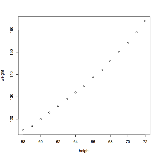
Plotting
> data(women)
> plot(women)
Plotting
use ggplot2Files?
m@x:~$ Rscript
Usage: /path/to/Rscript [--options] [-e expr [-e expr2 ...] | file] [args]
source('scriptname.R')
> HousePrice <- read.table("houses.data")
> HouseData <- read.csv("houses.csv")
Working With Data
TONS of Analysis and Statitical functionsWorking With Data
Taking a look:
> data(women)
> dim(women)
[1] 15  2
> names(women)
[1] "height" "weight"
Working With Data
Taking a look:
> head(women)
  height weight
1     58    115
2     59    117
3     60    120
4     61    123
5     62    126
6     63    129
> tail(women)
   height weight
10     67    142
11     68    146
12     69    150
13     70    154
14     71    159
15     72    164
Working With Data
Taking a look:
> summary(women)
     height         weight
 Min.   :58.0   Min.   :115.0
 1st Qu.:61.5   1st Qu.:124.5
 Median :65.0   Median :135.0
 Mean   :65.0   Mean   :136.7
 3rd Qu.:68.5   3rd Qu.:148.0
 Max.   :72.0   Max.   :164.0

> str(women)
'data.frame': 15 obs. of  2 variables:
 $ height: num  58 59 60 61 62 63 64 65 66 67 ...
 $ weight: num  115 117 120 123 126 129 132 135 139 142 ...
Working With Data
Distributions
rnorm: generate random Normal variates with a given mean and standard deviationdnorm: evaluate the Normal probability density (with a given mean/SD) at a point (or vector of points)pnorm: evaluate the cumulative distribution function for a Normal distributionrpois: generate random Poisson variates with a given rate
*norm, *pois, *binom, *gamma, ...
Working With Data
apply and family
# create a matrix of 10 rows x 2 columns
> m <- matrix(c(1:10, 11:20), nrow = 10, ncol = 2)

# mean of the rows
> apply(m, 1, mean)
 [1]  6  7  8  9 10 11 12 13 14 15

# mean of the columns
> apply(m, 2, mean)
[1]  5.5 15.5

# divide all values by 2
> apply(m, 1:2, function(x) x/2)
      [,1] [,2]
 [1,]  0.5  5.5
 [2,]  1.0  6.0
 [3,]  1.5  6.5
 [4,]  2.0  7.0
 [5,]  2.5  7.5
 [6,]  3.0  8.0
 [7,]  3.5  8.5
 [8,]  4.0  9.0
 [9,]  4.5  9.5
[10,]  5.0 10.0
see also lapply, tapply, sapply...
Packages
- Standard packages
-
CRAN!!
- > 6000 packages
- Graphics, Database Drivers, Machine Learning, Genetics, NLP, Spatial...
- swirl